Testing a Simple ARIMA Prediction Strategy

This past week we have been working on several traditional (simple, we could say) quantitative strategies looking for possible improvements from new angles. One such simple strategy is using regression models to predict market direction, basically using the past to predict the future.

Traditional market knowledge has it that "price only" cannot be used to predict future prices, prices are random, or have been traditionally handled in such a way that they are made apparently random. Marcos Lopez de Prado offers a very good discussion on the topic in his book "Advances in Financial Machine Learning" and in the Quantopian 2018 conference.

We are not going to use fractional differentiation (ARFIMA) in our model yet; in this post we will go through a traditional ARIMA model from conception to back-test in order to check if there is a single ray of hope for "price only" regression models.

As usual we are using a Quantconnect project to create and test our model.

First of all we will import the required modules and arrange our Jupyter Notebook output graphs:

import seaborn as sns

import matplotlib.dates as mdates

from pandas.plotting import register_matplotlib_converters

register_matplotlib_converters()

from IPython.core.display import HTML

#Center the plots in Jupyter Notebook:

HTML("""

<style>

.output_png {

    display: table-cell;

    text-align: center;

    vertical-align: middle;

}

</style>

""")

We will use the historical daily prices of Caterpillar (CAT) for our initial example. We will use historical data from 2010 to 2015 so that our ARIMA model research does not interfere with our backtest data from 2015 to 2020.

qb = QuantBook()

cat = qb.AddEquity("CAT")

start = datetime(2010,1,1)

end = datetime(2015,1,1)

history = qb.History(qb.Securities.Keys, start,end, Resolution.Daily)

The historical price looks like this:

plt.rcParams["figure.figsize"] = (16, 7)

plt.style.use('dark_background')

history.reset_index(inplace = True)

fig,ax1 = plt.subplots()

plt.plot(history['time'],history['close'])

plt.legend(['CAT Close Price'])

plt.ylabel('Price in dollars')

monthyearFmt = mdates.DateFormatter('%Y %B')

ax1.xaxis.set_major_formatter(monthyearFmt)

_ = plt.xticks(rotation=45)

We will use the Augmented Dickey-Fuller test to verify that the price series that we have for Caterpillar close prices is, indeed, non-stationary:

from statsmodels.tsa.stattools import adfuller

p_value = adfuller(history['close'])[1]

if p_value > 0.05:

    print("The p-value is: {p_value} > 0.05, hence time series is not stationary.".format(p_value=p_value))

else: 

    print("Time series is stationary.")

The result being as expected:

The p-value is: 0.08112394216397467 > 0.05, the time series is not stationary.

We are using just the statistic result from adfuller function, if we look at the full result of the adfuller() function the output is a tuple like this, with statistic and p-value on top:

(-2.6605133582666496,
 0.08112394216397467,
 14,
 1243,
 {'1%': -3.435621806786881,
  '5%': -2.8638680226791444,
  '10%': -2.5680094689100477},
 3910.193769373683)

We will also check how autocorrelated the price time series is. To verify that the autocorrelation between values is high we will use an autocorrelation plot:

from statsmodels.graphics.tsaplots import plot_acf

plot_acf(history['close'])

plt.xlabel('Lags')

plt.ylabel('Autocorrelation')

plt.show()

The time series is autocorrelated for a large number of lags. This and the ADF test confirm that our series is indeed non-stationary. What can be done to turn this series into stationary? We will assume that while the price values of a stock do not maintain constant statistical properties the series of price difference between two consecutive closes does.

We will plot the first order differential of the price series:

plt.plot(history['time'],history['close'].diff())

plt.xlabel('Date')

plt.legend(['First Order Difference'])

plt.show()

Now this differential time series does not obviously look non-stationary. In any case we cannot tell with total certainty if it is stationary or not just by looking at the plot. We will pass the new series through the ADF test and the autocorrelation test.

adfuller(history['close'].diff().dropna())

(-9.300785356251076,
 1.1139917377238033e-15,
 13,
 1243,
 {'1%': -3.435621806786881,
  '5%': -2.8638680226791444,
  '10%': -2.5680094689100477},
 3914.138290763847)

We verify that the statistic value and p-value are very low, low enough to indicate both a stationary time series and that possibly series memory has been lost, wiped. Marcos Lopez de Prado explains it in the conference video. The autocorrelation plot is now:

plot_pacf(history['close'].diff().dropna(), lags=20)

plt.xlabel('Lags')

plt.ylabel('Partial Autocorrelation')

plt.show()

We will use 80% of our data to train out model, we split the historical data into train, test and, although we are not going to use it today, embargo data.

split_point = 0.80

embargo = 0

split_train = int(len(history)*split_point)

split_test = int(len(history)*split_point+embargo)

train_set, test_set, embargo_set = history[:split_train], history[split_test:], history[split_train:split_test]

# Plot Train and Test set

plt.rcParams["figure.figsize"] = (16, 7)

plt.title('Caterpillar Stock Price')

plt.xlabel('Date')

plt.ylabel('Price in dollars')

plt.plot(history['time'][:split_train],train_set['close'], 'green')

plt.plot(history['time'][split_test:],test_set['close'], 'red')

plt.plot(embargo_set['close'], 'blue')

plt.legend(['Training Set','Testing Data'])

monthyearFmt = mdates.DateFormatter('%Y %B')

ax1.xaxis.set_major_formatter(monthyearFmt)

_ = plt.xticks(rotation=45)

plt.show()

Let´s now fit this training data set to our ARIMA model. In this case, after some very minor trials, the p and q values for the model will be 4, this values can be selected by looking for maximal values of Akaike Information Criteria and Bayes Information Criteria. This ARIMA model will be so simple that fine tuning these values a lot may result in undesirable overfitting. Using smaller p and q values has also the advantage of a faster computation, so that values of 2 for both p and q can also provide acceptable results. The "1" value in the middle of the ARIMA model order keyword argument is the order of differentiation we are using.

import warnings

warnings.filterwarnings("ignore")

from statsmodels.tsa.arima_model import ARIMA

p=4, q=4

model = ARIMA(train_set['close'], order=(p,1,q))

model_fit_0 = model.fit()

With this model in place we generate a rolling prediction for a single day for a few data points in the test data set. Take into account that we are feeding a real (actual) value after every day, so this model is limited to predicting the closing price tomorrow using the closing price today.

past = train_set['close']

predictions = []

pred_limit = 10

partial_test_set = test_set['close'][:pred_limit]

for i in partial_test_set.index:

    model = ARIMA(past, order=(p, 1, q))

    model_fit = model.fit(

        disp=-1, start_params=model_fit_0.params)

    forecast_results = model_fit.forecast()

    pred = forecast_results[0][0]

    predictions.append(pred)

    past[i]=partial_test_set.loc[i] 

predictions = pd.Series(predictions, index=partial_test_set.index)
for i in partial_test_set.index:

# Predicted and actual Values

for i in partial_test_set.index:

print('predicted={pred:.2f}, actual={test:.2f}'.format(pred=predictions.loc[i],test=partial_test_set.loc[i])

With the prediction for these days being:

predicted=74.65, actual=73.63
predicted=73.61, actual=73.57
predicted=73.52, actual=72.61
predicted=72.74, actual=72.85
predicted=73.00, actual=73.02
predicted=72.88, actual=73.50
predicted=73.65, actual=74.13
predicted=74.27, actual=73.65
predicted=73.58, actual=74.20
predicted=74.20, actual=75.71

Not a lot to be read from the numbers, these seem to be inside the sensible price range, something that can be considered and achievement in some cases. To gain more information on how these values for daily prediction deviate from actual recorded values we can compute the mean absolute percentage error:

def mean_absolute_percentage_error(y_true, y_pred):     

    return np.mean(np.abs((y_true - y_pred) / y_true)) * 100

mape = mean_absolute_percentage_error(partial_test_set, predictions)

print('Test MAPE: {mape:.2f}%'.format(mape=mape))

Test MAPE: 1.22%

Mean Absolute Percentage Error (MAPE) can be more easily understood in this price prediction context than the more usual Mean Square Error (MSE), where the error numbers will be large integers. In this case the function is custom made as sklearn does not have built in MAPE, it can very often generate divide by zero errors. Mean Absolute Error (MAE) is available providing a similar intuitively comparable value.

In any case we have a 1.22% error in our daily predictions for these 10 first values. Even if this prediction is not very accurate there may still be a directional prediction capability in the model that can offer positive returns as indicated by a simple prediction directionality test in these first 10 test cases.

for i in partial_test_set.index[:-1]:

    dir_predicted = predictions.loc[i+1] - partial_test_set.loc[i]

    dir_actual = partial_test_set.loc[i+1] - partial_test_set.loc[i]

    direction_predicted = np.sign(dir_predicted) == np.sign(dir_actual)

    print('Predicted Correct Direction={pred}'.format(pred=direction_predicted))

Predicted Correct Direction=True
Predicted Correct Direction=True
Predicted Correct Direction=True
Predicted Correct Direction=True
Predicted Correct Direction=False
Predicted Correct Direction=True
Predicted Correct Direction=False
Predicted Correct Direction=False
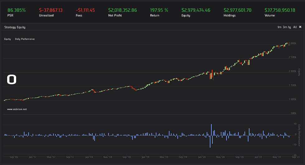
Predicted Correct Direction=True

In a very simple close-to-close algorithmic model the performance of the ARIMA prediction is enough to generate positive returns in a shaky 5 year period for Caterpillar.

This is a 7.3% Compounding Annual Return test, Sharpe ratio is very low at 0.4 and has a 32% drawdown at some point. The returns are very unevenly distributed, and our prediction is no better than a naive prediction.

We can also use Tesla (TSLA), a swing trader´s favourite, to test our model, to barely positive results:

If the behaviour of different companies can be characterized in time we could probably make a better use of the ARIMA model, we will have to add probably traded volume data to the model to gain better insights on the price action that the ARIMA model is trying to predict. In any case...

Not stellar results although it seems that with other additional prediction information built into the model (volume data, past price context) the ARIMA model would not be so grandly confused at some market reversals. The model is completely oblivious to past price memories (differentiation deletes them) that can probably be returned to the model as technical factors.

We think it is worth elaborating ARIMA models in the future, probably better if the model is AFRIMA, not to have to patch an ARIMA model to return lost price memory to it. For the time being remember that no information in ostirion.net constitutes financial advice, we do not hold positions in any of the companies or assets that we mention in our posts at the time of posting. If you are in need of asset management model development, deployment, verification or validation do not hesitate and contact us.