Mapping GEO Data with Folium

We extracted geographical information from a Web Features Service in our previous post and turned them into packaged CSV files for easy reading and re-reading. Today, we will represent these points of interest into a map we can use to display updated satellite imagery for information gathering purposes. In a follow-up post, we will extract these images for offline use when internet access is unavailable, or we do not want to add request load to free map tile serving services unnecessarily.

First of all, we need the location of the theoretical kilometer points we extracted in our previous work; if you do not want to run the previous notebook, you can download the file here:

PKTeoricos_ADIF

.csv

Download CSV • 1.14MB

This is just a 1 MB CSV text file with the index of a certain theoretical point in the railway network of Spain, with its location, network section to which it belongs, and the province it is located at.

We will first load these points, using pandas, into a data frame for easy manipulation, as this was the objective of all the preliminary digging and refining we did. We will need to import pandas and read the CSV file. The CSV file contains both a header with the column names in its topmost row, and the first column are the indexes of the kilometer points, so we pass the header and index_col keyword arguments to the CSV reader:

import pandas as pd
pk_data = pd.read_csv('PKTeoricos_ADIF.csv', header=0, index_col=0, dtype=str)

The shape of the resulting data frame should be something like this:

And note that the data type for the columns is "str", a string, as some data is numeric with leading zeroes that we will need to preserve. This makes our coordinate point data difficult to handle, and we must transform it into floating-point numbers. At the same time, we will set these values into a list to have a pair of floats for each coordinate point. We will use a single line to compensate for the ugliness of the code in our previous post. We will perform this transformation using a lambda function and list comprehension in a single go:

pk_data['numeric_coords'] = pk_data['coords'].apply(lambda x: [float(n) for n in x.split(" ")]) 

An innocent, although longish, line of code in which we apply to the data frame column a comprehension with transformation into float from the split string. Now, 'numeric_coords' contains a list with both geographical coordinates for all points.

There are 16,824 points in total. For demonstration purposes, we will focus our mapping on a specific section of the network; we will use section 061600120 as our "area of interest" (aoi):

aoi = pk_data[pk_data['section'] == '061600120'] 

We have seven points in this section, sufficiently few to rapidly map them into folium. We need some previous work to get folium maps to appear in a notebook environment properly. We will need to change the projection of our points from their EPSG25830 reference to the global reference system used by most global mapping tools, EPSG4326. This needs to be done to maintain the "flattening of the earth" we are trying to do. For more information on the complex topic of cartographic projection, this Wikipedia entry gives a good overview. For this, we import pyproj and folium; if using Google Colab, pyproj will need installing first:

!pip install pyproj
import folium
from pyproj import Proj, transform
# Coordinates change for this area:
inProj = Proj(init='epsg:25830')
outProj = Proj(init='epsg:4326')

This sets us up to plot the points in the area of interest. In this case, we will iterate over all the rows in the data frame in reverse to show first the last index point. The reason is just that we know this is where the train station is located. This first point will create the map, centered in the first location, at a given zoom level and window size for the map 50% of the full width. For subsequent points, we add a marker with the corresponding name of the point. The following snippet is best seen in the notebook at the end of the post due to the embedded conditions:

m_init = False
for index, point in aoi[::-1].iterrows():
    x, y = point['numeric_coords']
    x, y = transform(inProj,outProj,x,y)
    p_name = 'PK - ' + point['km_point']
    
    if not m_init:
        map = folium.Map(location= [y,x] , zoom_start=14, width='50%', 
        height='60%')
        folium.Marker(location=[y,x], popup=p_name, icon = 
        folium.Icon(color='yellow')).add_to(map)
        m_init = True 
        continue
   
folium.Marker(location=[y,x], popup=p_name, icon = folium.Icon(color='yellow')).add_to(map)
map

The results are a map with all the location of the points with their name in the pop-up, the points over the railway section going from Santander to Muriedas in Spain:

This map is constructed using Open Street Map tileset, containing the slowly changing layout of streets and installations. If we need to have actual images of the status of the infrastructure or location for our information gathering needs we are inspecting, we require access to satellite imagery. We can use a free-to-use service, from ESRI, for example, to plot our locations of interest in relatively low-resolution images such as these:

tile = folium.TileLayer(
      tiles = 'https://server.arcgisonline.com/ArcGIS/rest/services/World_Imagery/MapServer/tile/{z}/{y}/{x}',
      attr = 'Esri',
      name = 'Esri Satellite',
      overlay = False,
      control = True
      ).add_to(map)
map 

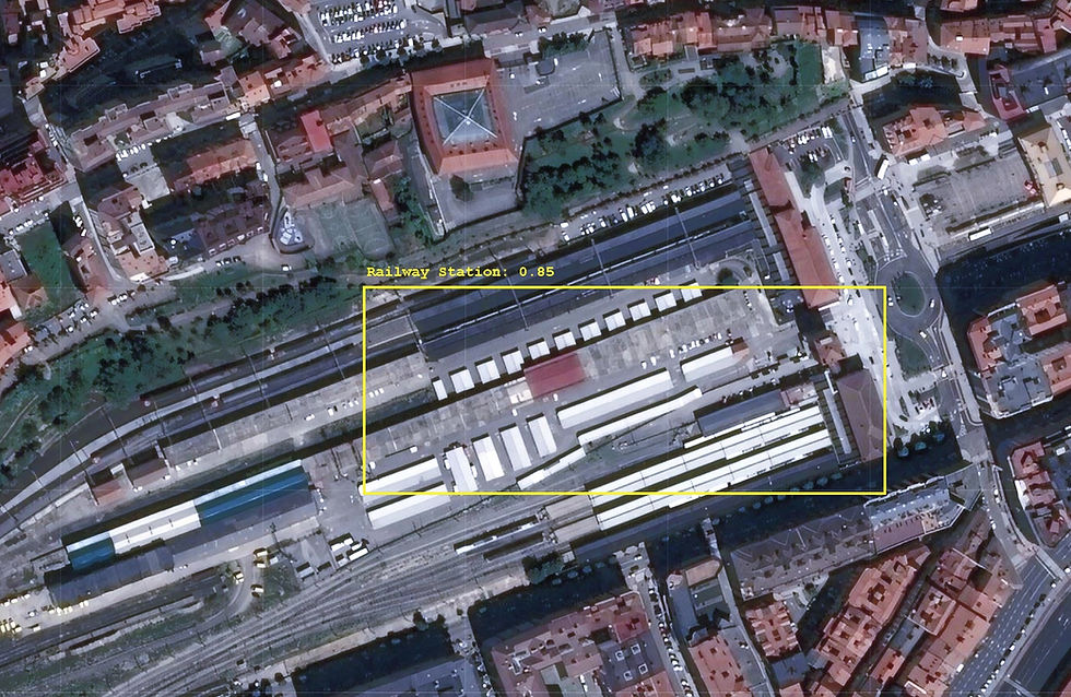
The maximum resolution we could use from this source if we were interested in the general state of the railway station in our area of interest would be something similar to this:

And this is not bad at all, although we will find the most interesting information in the images generated by commercial satellites at the 0.5m or 0.3m resolution. There is, of course, a cost associated with obtaining periodic images at such a high resolution. These high-cost images at the highest possible spatial and time resolutions will provide, in return, the maximum amount of economically actionable intelligence.

We will extract the spatial sequence of images for offline use and manipulation using these same mapping tools and satellite imagery in our next entry.

If you require quantitative model development, deployment, verification, or validation, do not hesitate and contact us. We will also be glad to help you with your machine learning or artificial intelligence challenges when applied to asset management, automation, or intelligence gathering from satellite imagery.

The notebook for this post is located in this Google Colab notebook.