All Tomorrow's Parties - Identifying Largest Market Moves Using Deep Learning (Part III)

In this third installment of our journey to predicting the largest market movers of tomorrow we are going to implement and improve a set of simple neural networks.

We are going to use these three previous components of our analysis:

1 - The setup of the symbols and dates that will be used for developing the model. This snippet can easily be modified to make use of the symbols we need. It is not important what symbols we use, as during backtesting the model will algorithmically select the symbols. This is just a sample for model development aimed at testing that the model itself can handle a large set of symbols (large being more than 2).

self = QuantBook()
start = datetime(2010,1,1)
end = datetime(2015,1,1)
# Random Choices from SP500 Tickers
tickers = ['GE', 'GT', 'BA', 'GM', 'V', 'MSFT', 'VZ', 'HD', 'CSCO']
symbols  = {}
for ticker in tickers:
    symbols[ticker] = self.AddEquity(ticker).Symbol

2- Cleaning up and reorganizing our history to obtain the features data and the target data:

daily_history = self.History(list(symbols.values()), start, end, Resolution.Daily).round(2)
daily_history['1D_Return'] = daily_history.groupby('symbol')['close'].pct_change(1).dropna()
daily_returns = daily_history[['1D_Return']].dropna()
daily_returns = daily_returns.unstack(0)
daily_returns.columns = daily_returns.columns.droplevel()
tops = daily_returns.idxmax(axis=1)
flops = daily_returns.idxmin(axis=1)
inv_map = {str(v.ID): k for k, v in symbols.items()}
np.vectorize(inv_map.get)(tops)
np.vectorize(inv_map.get)(flops)
symbol_idxs = set(daily_history.index.get_level_values(0))
targets = pd.DataFrame(0, index=tops.index, columns = symbol_idxs)
for date in targets.index:
    if daily_returns.loc[date,tops[date]]>0:
        targets.loc[date][tops[date]] = 1
    if daily_returns.loc[date,flops[date]]<0:
        targets.loc[date][flops[date]] = -1

targets.rename(columns = inv_map, inplace = True)
flops = targets.replace(1,0).replace(-1,1)
tops = targets.replace(-1,0)

3- Generation of the tensors that will be fed into our neural networks. The output of this snippet can also be easily modified to obtain different shapes of input tensors:

from operator import itemgetter as at
history = self.History(list(symbols.values()), start, end, Resolution.Hour).round(2)
history['index_values'] = history.index
raw_data = history
raw_data['date'] = history['index_values'].apply(at(1)).dt.date
raw_data['hour'] = history['index_values'].apply(at(1)).dt.time
raw_data.reset_index(inplace = True)
raw_data.set_index(['symbol','date', 'hour'], inplace=True)
features = ['close', 'volume']
raw_data = raw_data[features]
raw_data.reset_index(inplace=True)
samples = raw_data.set_index(['symbol', 'date', 'hour'])
samples = pd.DataFrame(samples.groupby(['symbol', 'date']).apply(lambda x: np.stack(x.values)))
samples.columns = ['Samples']
from sklearn.preprocessing import normalize, scale, MinMaxScaler

minmaxscaler = MinMaxScaler()
scalers = [lambda x: minmaxscaler.fit_transform(x),
           lambda x: scale(x,axis=0),
           lambda x: normalize(x,axis=0)]

scaled_samples = samples
use_n = 2
for lambda_f in scalers[0:use_n]:
    scaled_samples = pd.DataFrame(scaled_samples.Samples.apply(lambda_f))

scaled_samples = scaled_samples.applymap(lambda x: np.around(x,4))
samples = scaled_samples.reset_index().pivot(columns = 'symbol', index='date', values='Samples')
samples = pd.concat([samples, targets], axis=1).dropna()
samples['lens'] = samples[samples.columns[0]].apply(lambda x: len(x))
samples=samples[samples['lens'] == 7]
samples.drop(columns = ['lens'], inplace=True)
samples[targets.columns] = samples[targets.columns].shift(-1)
samples.dropna(inplace = True)
from sklearn.model_selection import train_test_split
dimensions = [-1]
test_size = 0.2
train, test = train_test_split(samples, test_size=test_size)
train_shape = (len(train),*dimensions)
test_shape = (len(test), *dimensions)

inputs = samples.columns[:len(symbols.keys())-1]
X_train = np.stack(np.concatenate(np.array(train[inputs].values))).reshape(train_shape)
y_train = np.array(train[targets.columns].values).reshape(len(train),-1)

X_test = np.stack(np.concatenate(np.array(test[inputs].values))).reshape(test_shape)
y_test = np.array(test[targets.columns].values).reshape(len(test),-1)

Starting from these tensors we analyze a deeper network than our original mini-model, for example a several layers deep network:

import tensorflow as tf
from tensorflow import keras
from tensorflow.keras import layers

n_out = len(targets.columns)

model = keras.Sequential([
        layers.Dense(18, activation="tanh", name="layer1"),
        layers.Dropout(0.2),
        layers.Dense(18, activation="tanh", name="layer1"),
        layers.Dropout(0.2),
        layers.Dense(18, activation="tanh", name="layer1"),
        layers.Dropout(0.2),  
        layers.Dense(18, activation="tanh", name="layer1"),
        layers.Dropout(0.2),  
        layers.Dense(n_out,activation='tanh')
    ])

history = model.compile(loss='mse', optimizer='adam', metrics=['mse'])

The model can be trained for a given number of epochs that can be used to define the patience of the model through keras callbacks:

EPOCHS = 50
patience_rate = 0.1
patience = int(EPOCHS*patience_rate)

callbacks =  tf.keras.callbacks.EarlyStopping(monitor='val_loss', patience=patience)
model.fit(X_train, y_train, epochs=EPOCHS,  validation_data=(X_test, y_test), callbacks = [callbacks])

Training deeper models will require longer times, in this case the training takes 10 minutes in a normal workstation with no GPU use. Before deploying the model it will have to be trained with 10 times more data so that we will be looking at several training hours per training cycle in any minimally useful environment. The model will ultimately be trading live and ideally training every few days. As long as a machine learning model takes less 48 hours or less to train, its training can safely be slotted in non-trading time frames, for stock market for example, or in low volume time periods for continuous market models as in foreign currency exchanges or cryptocurrency markets.

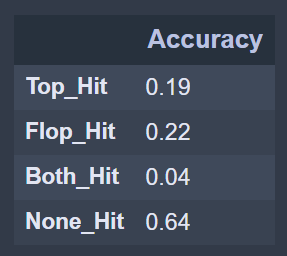
The accuracy performance of this "deeper" model is:

We have 10 symbols, we can select the top or the flop 20% of the time, the model predicts both almost 5% of the days, and none of them 64% of the days. There seems to be a small accuracy lift from the predictive power of the model. We are better off than randomly selecting a stock from the set to be the top or the flop. These capabilities will only be verified with the validation backtest, when the model sees completely new data is the largest possible market group. We will use this accuracy table as a baseline for a new model, lets see what happens if we make our model first deeper, wider and then both.

Deeper models can be constructed using the add method of Keras sequential models. This can make our models growth dangerously easy to implement. By iterating over a range we can add as many layers as wanted (possible not needed). The model is finally capped with the output layer with the number of target columns we need:

n_out = len(targets.columns)
n_layers = 60
model = keras.Sequential([])

for i in range(n_layers):
    model.add(layers.Dense(18, activation="tanh", name="layer1"))
    model.add(layers.Dropout(0.2))

model.add(layers.Dense(n_out,activation='tanh'))

This model now requires 2 minutes per epoch to train. There is a larger number of parameters to be learned that hopefully lead to a better description of the prediction problem that will, sadly, also lead to overfitting for this specific time frame and symbol set. Our overarching assumption is that local improvements in model predictive power can be expanded to other periods and symbols, that the market will behave with a relative similarity regarding its largest movers across time and stocks.

Training this model yields a noticeable degradation. The fitting of the parameters occurs in fewer epochs, 9 epochs are enough to reach the following test accuracy, apparently with a large overfitting:

We now change the shape of the network in the other dimension, we can set up some code to easily modify the width of the network and check whether our validation accuracy can be improved:

n_out = len(targets.columns)
n_layers = 5
width = 100
model = keras.Sequential([])

for i in range(n_layers):
    model.add(layers.Dense(width, activation="tanh", name="layern"))
    model.add(layers.Dropout(0.2))

model.add(layers.Dense(n_out,activation='tanh'))

history = model.compile(loss='mse', optimizer='adam', metrics=['mse'])

This is the result for a wider network, there is not a lot of improvement either:

This is a probable case of large overfitting in the initial layers of the neural network. One of the simplest methods to avoid this overfitting is a large first layer dropout rate. This paper contains a very good discussion on the topic of overfitting and dropout in problems that are more complex that ours.

The target is now to find a combination of depths and widths for a simple neural network that can yield the best out of sample accuracy. By iterating over combinations of depth and width for these simple neural networks we can find an optimum set of hyperparameters that yields the lowest "no hit" metric. To prevent the very high overfitting that the first layer of the model will incur into we can also add a larger dropout value for the model:

n_out = len(targets.columns)
n_layers = 5
width = 100
model = keras.Sequential([])
model.add(layers.Dense(width, activation="tanh", name="layer1"))
model.add(layers.Dropout(0.8))

for i in range(n_layers):
    model.add(layers.Dense(width, activation="tanh", name="layern"))
    model.add(layers.Dropout(0.2))

model.add(layers.Dense(n_out,activation='tanh'))

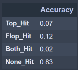
This will be our first simple neural network model. We are expecting to correctly predict either the top or the flop (or both) 38% of the days in a 10 stock market. Lets double the number of stocks by picking random SP500 entries again and checking how a larger field of possible tops and flops affects the relative prediction accuracy:

We can consider this our baseline neural network model now as apparently the relative predictive power is maintained. The most sensible approach is to implement this model in a backtesting environment and check that the predictions hold, in relative accuracy terms, when presented with new data. The predicted operations will indeed need to outperform the random selection of stocks and turn out a profit for the model to be considered useful and deserving of further development. This will be the topic for our next publication.

Remember that information in ostirion.net does not constitute financial advice, we do not hold positions in any of the companies or assets that we mention in our posts at the time of posting. If you are in need of algorithmic model development, deployment, verification or validation do not hesitate and contact us. We will be also glad to help you with your predictive machine learning or artificial intelligence challenges.