Price Time Series: Statistical Decomposition for SPY Price & Prophet

We like Prophet, we liked Image Comics Prophet revival a lot. Prophet is also Facebook's "free" time series forecasting tool, "free" in big tech usually being: "you are the product". This is the Prophet repository and this is its quick start guide. The starting guide is very good and shows how the API simplifies time series testing and forecasting. It uses the same model-fit-predict approach that sklearn does. We will try to use this tool to obtain stock market price forecasts as it claims can discover non-linear trends. It also appears to be good at detecting seasonality, a property our stock market price data may not exhibit, or is very weak, from our previous post.

We will use our previous work and create a new function to obtain a time series from Quantconnect history call, for a single symbol for the time being:

import matplotlib.dates as mdates
import matplotlib.pyplot as plt
import numpy as np

self = QuantBook()
spy = self.AddEquity("SPY")
history = self.History(self.Securities.Keys, 365*5, Resolution.Daily)

def create_plot(x, y, color='blue', size =(16,7), legend='Close Price', y_label='Price in USD' ):     
    plt.style.use('dark_background')
    plt.rcParams["figure.figsize"] = size    
    fig,ax1 = plt.subplots()    
    plt.plot(x,y, color=color)
    plt.legend([legend])
    plt.ylabel(y_label)
    date_form = mdates.DateFormatter("%m-%Y")
    ax1.xaxis.set_major_formatter(date_form)
    start, end = ax1.get_xlim()
    ax1.xaxis.set_ticks(np.arange(start, end, 90))
    _=plt.xticks(rotation=45)

def create_time_series(df, column='close', freq='d'):
    df = df.reset_index()
    time_series = df[[column]].set_index(df['time']).asfreq(freq).ffill()
    return time_series

Prophet can be imported without additional work, as it is part of Quantconnect supported libraries:

from fbprophet import Prophet 

We want to create a model, the simplest way being:

price_model = Prophet()

There are a bunch of options not in the quickstart guide, so a help(Prophet) reveals to us that we may specify, among other things linear or logistic trends, the chance to fit or not to fit different seasonalities and the uncertainty intervals. For this first model we will keep ourselves to the defaults, later we can always torture the model in the rack of a grid-search until it predicts well.

Prophet requires a very specific format for the time series, a serial index, a ds column with the dates and a y column with the target variable:

time_series.reset_index(inplace=True)
time_series.columns = ['ds', 'y']
price_model.fit(time_series)

The model is fit to our past SPY price data, now, to generate a prediction we have to generate a future dataframe. Let's predict 5 days into the future since our last available value, the value for today. This is just a trial to check that the model can work:

price_forecast = price_model.make_future_dataframe(periods=5, freq='d')
price_forecast = price_model.predict(price_forecast)

It takes a while to predict the next five days for SPY, we obtain a nice graphical representation of the model with built-in plotting tool, we modify here the color template as our preferred dark style does not work well with Prophet default colors:

_=plt.style.use('seaborn')
_=price_model.plot(price_forecast, xlabel = 'Date', ylabel = 'Price', figsize=(12, 6))

The plot show the observed values as dots, the trendline and the upper and lower bounds of the combination of trend prediction and seasonalities. The prediction generates quite a wide dataframe with these columns:

Index(['ds', 'trend', 'yhat_lower', 'yhat_upper', 'trend_lower', 'trend_upper',
       'additive_terms', 'additive_terms_lower', 'additive_terms_upper',
       'weekly', 'weekly_lower', 'weekly_upper', 'yearly', 'yearly_lower',
       'yearly_upper', 'multiplicative_terms', 'multiplicative_terms_lower',
       'multiplicative_terms_upper', 'yhat'],
      dtype='object')

The prediction we are seeking is 'yhat'. We can find what the prediction is for the next five days:

pred_true = price_forecast[['ds','yhat']].join(time_series[['y']])
pred_true.set_index('ds', inplace=True)
pred_true.iloc[-10:]

The prediction seems to be operational, predicting slightly growing SPY prices for next week, through the second weekend of November. We can check with this information if this type of modelling shows any promise. We translate this research into a simple backtest algorithm, we will try to predict the price of SPY five days (a random starting point) ahead into the future and enter positions accordingly.

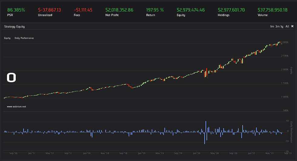
The results are surprising, the model can pick up price reversals and manages to stay afloat in the period 2015 to 2020. Its generates a yearly 7.5% with a Sharpe ratio of 0.4. Not bad for a machine with zero tuned parameters:

It is very interesting that during this mainly bullish period the model has a preference for short positions, and is capable of navigating, somehow, the COVID19 period:

The 2018 to 2020 period is quite good, it steals a 5% additional return to the SPY hold strategy. It still generates a large quantity of short positions, even in a clearly bullish market.

Where are these predictions coming from? We cannot answer as we have not dived deep into the code for Prophet, it appears it may be worth checking what it is doing internally, there is some predictive power being generated there. Externally we can obtain a report for our model components:

_=plt.style.use('seaborn')
_=price_model.plot_components(price_forecast)

So, are there hidden seasonal patterns, or is it a trick of the light? If the case is for the seasonal effects that the model will find , be there or not, our best bet for further research is finding stocks with historically high seasonal components. There seems to be no conclusive publications on the matter of specific sector or stocks seasonality, so before embarking in a possibly futile quest for a statistically seasonal company we will try with a variable that should exhibit some seasonality: treasury bonds. We try our simple Prophet model on TLT US treasury bonds ETF, based in a super fast, non-exhaustive research:

The results are not stellar in terms of equity lost through a relatively safe asset, the directionality of the predictions is good at 55% hit rate. Given these results it is worth to gain a deeper understanding on Prophet calculation procedures. It is possible also worth researching more; the possibilities include finding really historically seasonal assets and treating the time series through fractional differentiation in an attempt to better capture repeating patterns.

Remember that information in ostirion.net does not constitute financial advice, we do not hold positions in any of the companies or assets that we mention in our posts at the time of posting. If you are in need of algorithmic model development, deployment, verification or validation do not hesitate and contact us. We will be also glad to help you with your predictive machine learning or artificial intelligence challenges.

Here is the research and backtesting code used in this post, for the TLT case: