Price Time Series: Statistical Decomposition for SPY Price & ARIMA Grid

There are multiple publications on the network (vast and infinite) regarding statistical analysis of time series using Python and its modules. In this publication series we will replicate the most common statistical analysis and inference tools and apply them to stock market price time series for several assets and resolutions. The goal is, of course, to find a predictive power edge beyond a naive model and anticipate market moves as this is the first step for the development of a profitable trading or asset management strategy, the ultimate source of alpha.

We are using Quantconnect´s research environment for this statistical demonstration. First of all we are going to obtain the history for the past 5 years of prices for the SPY index in a daily resolution:

self = QuantBook()
spy = self.AddEquity("SPY")
history = self.History(self.Securities.Keys, 365*5, Resolution.Daily)
history.reset_index(inplace = True)

To better take a look at the time series we obtained with this request we can define a handy plot function to customize the colors and sizes we prefer:

import matplotlib.dates as mdates
import matplotlib.pyplot as plt
import numpy as np

def create_plot(x, y, color='blue', size =(16,7), legend='Close Price', y_label='Price in USD' ):     
    plt.style.use('dark_background')
    plt.rcParams["figure.figsize"] = size    
    fig,ax1 = plt.subplots()    
    plt.plot(x,y, color=color)
    plt.legend([legend])
    plt.ylabel(y_label)
    date_form = mdates.DateFormatter("%m-%Y")
    ax1.xaxis.set_major_formatter(date_form)
    start, end = ax1.get_xlim()
    ax1.xaxis.set_ticks(np.arange(start, end, 90))
    _=plt.xticks(rotation=45)

So we can plot all our time series by calling this function given the x and y values we want to show:

x = history['time']
y = history['close']
create_plot(x,y, legend = 'SPY Close Price')

We know this time series is non-stationary, our statistical inference tools will be hard pressed to obtain long range predictions under this changing mean and variance environment. The form is not good. The good statistical forms are found in differentiated series, fractional or integer. For the most common integer differentiation, the shape, showing good statistical properties but no memory, is:

y_prime = y.pct_change()
create_plot(x,y_prime, legend = 'SPY Price Change')

We can further analyze the form of our time series data by using a method called time-series decomposition from statsmodel library. First we need to create a time series out of our resetted history dataframe:

time_series = history[['close']].set_index(history['time']).asfreq('d').ffill()

We have to construct a time series with a frequency different to 'None', in this case our frequency is daily but weekends and days in which the market is closed are marked as not available (NaN), we have to fill them forward to simulate that during the weekend or market closed periods the price stays as it closed the previous trading day, this is not totally correct but still valid for our analysis. We can now plot the time series decomposition to observe the trend, seasonality and residuals:

decomposition = sm.tsa.seasonal_decompose(time_series, model='additive')
plt.rcParams["figure.figsize"] = (10,10)
fig = decomposition.plot()
plt.show()

In the decomposition we can see the original series at the top, the strong trends below it, then the lack of seasonal patterns in the period and the residual, or error with respect to the trend. The trend is clearly of increasing prices from 2014 to 2020, a strong bull market. The periods of correction appear as high residual error in the residuals plot, and these show strong clustering in the periods of correction.

It is interesting to see the effect of the COVID19 crisis on the SPY price trend when compared to previous crisis periods. If we extend our history to the past 20 years we observe this decomposition:

The effect of the COVID19 trend breaking is much more noticeable than the dotcom bubble crisis, the 2008 subprime crisis and the 2015 mini-crisis. The impact of the global pandemic is a large dent on the trend, or the trend starting on 2012 has been exaggerated by external economic factors and makes this event especially noticeable.

The effect of this last crisis could be exaggerated from both sides: by the global, far-reaching impact of the pandemic and the abnormal exuberance from the 2012-2020 period. These values are not adjusted for inflation and thus mask the effective purchasing power effect of the crisis events, the effect is still large even after computing the adjusted price using approximate inflation values:

This decomposition we have is normally used to fit time series to ARIMA models (AutoRegressive Integrated Moving Average) with the intention of obtaining future predictions that take into account the trend of the price, the seasonality (lack of it in the case of stock prices in general) and the residual deviation from the moving average as noise. We tested a very simple ARIMA strategy in this post, we are expanding on the topic now with a more elaborate parameter selection. Increasing RANGE will increase the parameter grid size for our models, then we try each of these parameters for a solution, if there is no solution we continue to the next parameter, if there is a solution we record the Akaike Information Criterion metric as a performance metric for the resulting model:

import itertools
RANGE = 5
p = d = q = range(0, RANGE)
pdq = list(itertools.product(p, d, q))

y = time_series['close']
AIC_results = {}

for param in pdq:
    try:
        mod = sm.tsa.ARIMA(y, order=param)
        results = mod.fit()
        print(f'ARIMA{param} - AIC: {results.aic:.2f}')
        AIC_results[results.aic] = param
    except:
        continue

For this time series a range of 5 is probably too large, large ranges will take a very long time to test for convergence and fit. In this specific short history fitting the best model is found from the results dictionary:

best_params = AIC_results[min(AIC_results.keys())]

This parameter set is used to fit a single (locally best) model and obtain the summary parameters:

best_model = sm.tsa.ARIMA(y, order=best_params)
best_results = best_model.fit()
print(best_results.summary().tables[1])

Generally speaking P>|z| values above 0.05 indicate an "unreliable" parameter, so our model seems to be able to fit well the 2015 to 2020 SPY price periods. If we follow the same procedure to fit the 2000 to 2020 period the same summary table contains the following parameters for the best model according to the Akaike Information Criterion:

Seems also surprisingly good and we may have a case of full-fledged overfitting to the past. How well does the model predict the future? Built-in into tsatools plot_predict allows us to plot the time series values over a range of predictions to check how well the model can chase the real values:

start = datetime(2020, 1, 1)
end = datetime(2020, 1, 20)
plt.style.use('dark_background')
plt.rcParams["figure.figsize"] = (16,10)
pred = best_results.plot_predict(start, end, dynamic=False)

This shows the static forecast (as "dynamic" option is False) and shows the 1 step prediction for the given period. The model is quite capable of chasing this value, with ta few but performance-destroying predictions in which the directionality of the next day is wrongly predicted, when the forecast and the close lines cross.

The dynamic option lets us use the ARIMA model to predict several time-steps using the forward walking prediction results. Any prediction of significant length will accumulate a large error as more and more data points are predicted with more and more stale price data. As an example we can try to predict 15 days in the future dynamically from 2020-10-1 to 2020-10-16 for a very poor price prediction:

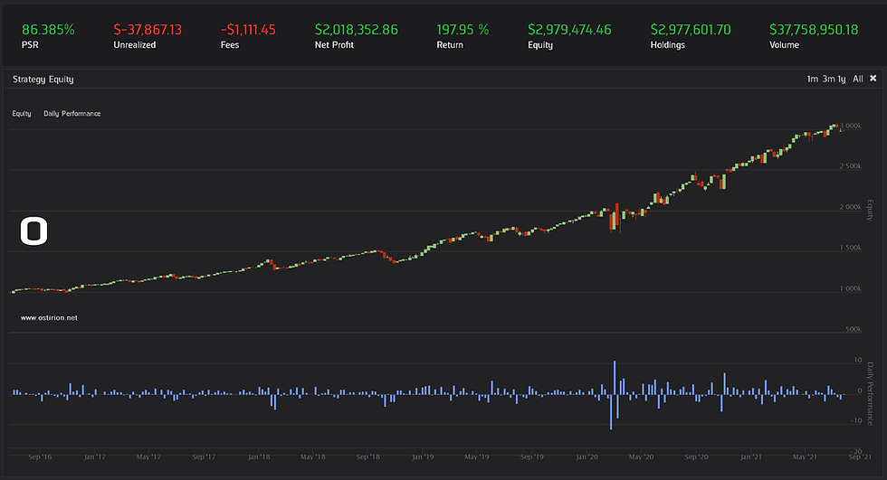
How will this more advanced ARIMA model behave under test? Let's see the results of a backtest in which we enter daily positions into SPY depending on the direction predicted by the ARIMA model and hold it for the day. The backtesting algorithm will look for optimal pdq values every 60 predictions and is limited to a grid range of 5 to obtain a relatively quick test:

The model has a very hard time obtaining correct predictions, we know that the price series is non-stationary and is forcing the ARIMA fit into many erroneous reversal traps. It shows a tendency for price reversals and favors short positions mostly. The ARIMA model picks up very well large drops and keeps on trying to catch drops in strongly bullish markets, making errors that cost us our little profits. At a yearly return rate of 4.4% and a sharpe ratio of 0.31 this ARIMA model does not help us much. A slow bleed during bull markets.

The first approach that we can use to fix this fitting problem is using fractionally differentiated price values as our time series. We can also use other prediction methods, Facebook Prophet, for example, even if it gives us the chills, we fear we may be the product. We will cover these approaches in future publications.

Remember that information in ostirion.net does not constitute financial advice, we do not hold positions in any of the companies or assets that we mention in our posts at the time of posting. If you are in need of algorithmic model development, deployment, verification or validation do not hesitate and contact us. We will be also glad to help you with your predictive machine learning or artificial intelligence challenges.