Price Time Series: Fractionally Differentiated Series with Prophet
- H-Barrio

- Nov 17, 2020
- 6 min read
In our previous post in this series we noticed that Facebook´s Prophet time series statistics tool can potentially generate decent predictions for carefully researched stocks under certain circumstances. Before launching ourselves in a wide array search for highly seasonal, quasi-stationary financial instruments we can force a stationary series out of the price of any instrument, in this case, for the sake of simplicity, SPY.
We will use MLFInlab fractional differentiation module (as we did here) to obtain the "best" fractional series and apply Prophet fitting and prediction to it. We will keep it to a 5 day prediction for the time being, ideally, and after forcing the machine to do a lot of work, the best prediction windows for each season could be found, with the risk, of course, of local overfitting to past data.
No changes to the initial part of our process with respect to our previous post on FB Prophet:
import matplotlib.dates as mdates
import matplotlib.pyplot as plt
import numpy as np

self = QuantBook()
spy = self.AddEquity("SPY")
history = self.History(self.Securities.Keys, 365*5, Resolution.Daily)
A little improvement on the time series generation function in Prophet format, so that the output fits right away into the model:
def create_time_series(df, column='close', freq='d'):
    df = df.reset_index()
    time_series = df[[column]].set_index(df['time']).asfreq(freq).ffill()
    time_series.reset_index(inplace=True)
    time_series.columns = ['ds', 'y']
    return time_series
With this, just create a time series for the current symbol, still SPY:
time_series = create_time_series(history)With the time series created, the best fractional difference can be found, that is, the lowest value of d that gets the series through the augmented Dickey–Fuller test:
from mlfinlab import fracdiff
from statsmodels.tsa.stattools import adfuller

fracdiff_values = np.linspace(0,1,11)
symbol_list = ['SPY']
fracdiff_series_dictionary = {}
fracdiff_series_adf_tests = {}
for frac in fracdiff_values:
    for symbol in symbol_list:
        frac = round(frac,1)
        dic_index = (symbol, frac)
        fracdiff_series_dictionary[dic_index] = fracdiff.frac_diff(time_series[['y']], frac, thresh=0.1)
        fracdiff_series_dictionary[dic_index].dropna(inplace=True)
        fracdiff_series_adf_tests[dic_index] = adfuller(fracdiff_series_dictionary[dic_index])
The dictionary series are there to be used, if needed, in the future. We only need the "best" differentiated time series:
stationary_fracdiffs = [key for key in fracdiff_series_adf_tests.keys() if fracdiff_series_adf_tests[key][1] < 0.05]
first_stationary_fracdiff = {}
diff_series = {}
for symbol, d in stationary_fracdiffs:
    ds = [kvp for kvp in stationary_fracdiffs if kvp[0] == symbol]
    first_stationary_fracdiff[symbol] = sorted(ds, key=lambda x: x[1], reverse=False)[0][1]
    diff_series[symbol] = fracdiff_series_dictionary[(symbol, first_stationary_fracdiff[symbol])]
    diff_series[symbol].columns = ['diff_close_' + str(symbol)]

for symbol in symbol_list:
    print("The lowest stationary fractionally differentiated series for ", symbol, " is for d=",
          first_stationary_fracdiff[symbol], ".")
The message at the end of the block tells us that in this case the best fractional differential series occurs for d=0.3. In the backtest algorithm we will let this be calculated every prediction cycle, so it will be worth it to remove the dictionary storage and keep only the first series that fulfills the ADF test criterion. The resulting differentiated series has to be reformatted into a the Prophet 'y'-'ds' format again:
diff_time_series = diff_series['SPY'].join(time_series['ds'])
diff_time_series.columns = ['y', 'ds']
diff_time_series
The time series "indexes" and the differential values are aligned in this case. The weight thresholding function used to obtain the fractional differential series "uses up" some of the information that does not make it into the final series. The points that are lost are shown in the series table:

In the date table above, as we have requested 1825 points of data, the first value for 'ds' should be 2013-08-15. A threshold of 0.1 suppresses the first 36 points of data. This is not a problem for time series for which we have enough data, for shorter time series it may reduce the amount of data points critically to the point that no model can reliably be fitted with so little data.
The effect of changing the weight thresholds are interesting, shorter time series are obtained while extremely weighted points are dropped. In the future we will explore this effect, for the time being the explanation is in Marcos Lopez de Prado´s Advances in Financial Machine Learning book (page 80 and on). In any case the shape, the familiar shape, of a memory-optimal stationary series is this:

We can now generate the Prophet model by feeding it the differentiated time series, no changes here, no options whatsoever in an attempt to check how it can work with this new series out of the box, we also predict 5 days, no more thought given to it:
from fbprophet import Prophet
price_model = Prophet()
price_model.fit(diff_time_series)
price_forecast = price_model.make_future_dataframe(periods=5, freq='d')
price_forecast = price_model.predict(price_forecast)
And the aspect of the fit:
_=plt.style.use('seaborn')
_=price_model.plot(price_forecast, xlabel = 'Date', ylabel = 'Price', figsize=(12, 6))
The aspect is still good. The know past SPY behaviours are reflected in the time series and it is also stationary. Note the apparently strong mean reversion effect in the shorter term being maintained for most of the series until COVID19 crisis volatility creates a completely wild cloud of points out of the maximum and minimum bands predicted by the Prophet fit. This may be worth further investigation, if finally Prophet does not produce and accurate price movement prediction always, it may be able to do so reliably when trading happens at extremes out of the minimum and maximum prediction bands. In any we can use this model now to produce a 5 day SPY prediction using a dynamic best fractional differential selection. The results are:

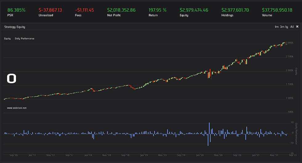
A little bit worse returns than for the raw price data model, returns are in any case more consistent now, with a 54% correct direction prediction. The model is not very intelligent and lacks any risk management capabilities, still the results can be considered not bad as the machine is not ruining itself. Also not good, as a SPY buy and hold strategy netted 86% return during the same period.
Is a 5-day prediction too long of a prediction? Do we have a too large of a horizon in this model? Too short? Note that we are not calculating the fractional integral to obtain a price level again, we are just comparing the differential direction to obtain a price direction. This is true for almost all cases, the fractional differential change will have the same direction as the price change, this breaks down for small differential price changes below the threshold that generate erroneous signals. With additional work the model could be modified to not act, to not take the shot, if the predicted change for the fractional differential value is below a certain threshold.
We can check the predictive capacity for 2 alternate prediction times, 3 days ahead, and 15 days ahead to learn something about the shape of a very short term prediction and a medium term prediction, first for the short term, with a 3 ahead directional prediction:

For 15 days ahead:

Both generate worse predictions, probably these periods lie in between the weekly and the monthly "seasonal" effects Prophet is trying to fit to with little success. The directionality is also not good in these models, with 46%-48% correct directionality. There seems to be no low hanging fruit from Prophet and fractional time series.
We can still try a final easy test, let's add a few more tickets to our universe, instead of focusing on predicting SPY, and accepting the full risk, we will pick the top 10 stocks by traded volume every prediction cycle, for a 5 day window, and see if it provides a better risk control. The full fractional differential and the full Prophet fit will happen every prediction cycle, so the model takes quite a while to complete the test: more than 24 hours as it differentiates and trains Prophet models every 5 test days:

At 51% correct direction predictions and at a 40% loss these wild, multiple Prophet models do not appear to work well together out of the box. Another approach is necessary, even if Prophet gives a prediction edge, the model is too naive in terms of the portfolio it tries to build. The market risk is apparently all there to trap us in our seasonal preferences.
As a final wild guess; what if we fit a shorter training model into cryptocurrencies? Let's see the same Prophet out-of-the-box model fitted to BTC USD history. We will start in 2018 has there is no reliable data to fit the model before that:

Does not look good.
It seems, by looking at all these simple models, that Facebook Prophet could be used to support price direction predictions, it will require a deeper dive into the calculation code and the algorithmic selection of instruments that exhibit certain characteristics. Out of the box application and popular instruments together do not offer good results. We have to keep on searching.
Remember that information in ostirion.net does not constitute financial advice, we do not hold positions in any of the companies or assets that we mention in our posts at the time of posting. If you are in need of algorithmic model development, deployment, verification or validation do not hesitate and contact us. We will be also glad to help you with your predictive machine learning or artificial intelligence challenges.


Comments