Predicting Volatility: Support Vector and Random Forest Classifiers
- H-Barrio

- Aug 18, 2020
- 5 min read
Continuing with the development of our VIX predicting machine learning model we have adapted the model to the backtest engine in Quantconnect. We are trying to predict the direction that the VIX indicator will move to at market close 5 days from today using as factors:
1- The fractionally differentiated SPY price history.
2- The VIX index level history.
Our model takes the least differentiated SPY price series that still results in a stationary time series and VIX index level, this is by itself stationary in the 5 year periods we are using. At this point we are only using these features, this model is basically an autoregression on VIX supported by SPY fluctuations.
We cannot directly trade volatility, being the simplest instrument to do this the ETFs that track the VIX index. As we are predicting a future time frame of 5 days VIXY appears to be the most suitable of the ETFs to mimic the direction of VIX. There are other, more complex methods, to trade on volatility involving option spreads and net volatility. If the VIX prediction shows promise this alternative method of profiting from the prediction could be used. This is a common theme in quantitative trading, you may have a decent prediction and need an instrument to trade on that prediction, and generally this is not straightforward and generates several problems of its own.
In our model we have to add SPY and VIXY as instruments, and VIX as data, through Quantconnect custom data import:
# CBOE data connection import:
from QuantConnect.Data.Custom.CBOE import CBOE
# Add Required Symbols
        spy = self.AddEquity('SPY', resolution).Symbol
        vix = self.AddData(CBOE, 'VIX', Resolution.Daily).Symbol
        vixy = self.AddEquity('VIXY', resolution).Symbol
We will be using, initially, the past 22 days to predict the direction of VIX 5 days from today:
# Prediction horizons need to pass from train to predict.
# So they are made part of the alpha model.
self.N_days_prediction = 5
self.lookback_window = 22
The update method for this alpha model contains the initial training and retraining of the model. This can be used to save time during the backtesting phase, as the model will have plenty of time during live operation to perform this training. Initially we will retrain the model every 31 days, at the end of the week, in the middle of the trading day where it will not interfere with the rest of the algorithm. The algorithm takes the decision to trade a 9:35 and will close the position at the close of the fifth day (N-1 days, as 9:35 marks the start of day 1). While we hold our instrument for the following 5 days we skip new predictions for the sake of simplicity. The prediction function performs all the input data transformation work, it has to re-differentiate the SPY close prices and reescale and normalize all values using the training model scaling variables. At this stage we are also predicting the past and we could obtain a dynamic evaluation of the model itself to be used for additional learning if the simple model proves useful.
def Update(self, algorithm, data):

        insights = []
        if not data.HasData: return []

        #Train the model every training cycle before market close:
        if self.trained == False or (algorithm.Time.month==self.next_month and algorithm.Time.weekday()==4 and algorithm.Time.hour==11 and algorithm.Time.minute==30):
            #Try using algorithm.Train():
            self.ML_model = self.train_model(algorithm, self.predictor, self.prediction_target)
            self.next_month = (algorithm.Time + timedelta(days=31)).month
            algorithm.Debug("Model Trained:" + str(algorithm.Time.year) +"-"+ str(algorithm.Time.month))
            self.trained = True

        if algorithm.Time.hour == 9 and algorithm.Time.minute == 35:
            if algorithm.Portfolio.Invested: return []
            hours = algorithm.ActiveSecurities[self.predictor].Exchange.Hours
            insight_duration = hours.GetNextMarketClose(algorithm.Time + timedelta(days=self.N_days_prediction-1), False) - algorithm.Time
            prediction = self.predict(algorithm)
            if prediction == 0: direction = InsightDirection.Down
            if prediction == 1: direction = InsightDirection.Up
            insights.append(Insight(self.instrument, insight_duration, InsightType.Price, direction, 0.02, 1, "MLVolatilityPrediction", 1))
            return insights

        return[]
We are not sharing the adaptation of the train and predict functions from the previous post, the reason being that it is mostly reused code from a LSTM model that is unnecessarily complicated when used with our current Support Vector Classifier model. It is doing the same again but goes back and forth with the dimensionality of the input arrays.
The first backtest run yields the following mixed results:

The predictive power of the model varies greatly with time. The results would have been bad, not mixed, if no pattern could be observed in the backtest results. It is apparent that there is some "seasonality" or market regime that we have not taken into account in our factors, we have just 2 factors with 22 days of past data. It is more apparent that something could be done to the model in the key performance indicator data:

The model favors long positions and stays for a long while in the high 60% directionality score, then the missing variables appear and reduce the direction score and the equity performance. The insights themselves are barely losing money, so there is probably something that can be done. Quick trials for drawdown control, VIX level limits or probability prediction cut-offs do not offer any better results.
It is a possibility that our support vector machine classifier is overfitting to data. We do not have a simple solution to this problem at this time, in order to verify this we are going to fit this model using the best fracdiff to a random forest classifier to verify the importance of the features, that is, past data points in the model.
After a random grid search for optimal parameters and a recursive feature elimination using cross validation (RFECS) we obtain this model:
best_rf_parameters = {'n_estimators': 400,
'min_samples_split': 5,
'min_samples_leaf': 1,
'max_features': 'sqrt',
'max_depth': 30,
'bootstrap': True}
best_random_forest = RandomForestClassifier(**best_rf_parameters)
rfecv = RFECV(estimator=best_random_forest, step=1, cv=tscv,
              scoring='accuracy', verbose=2)
rfecv.fit(X_train_windows, y_train_windows)
The best parameters for a testing accuracy of 54% are, surprisingly, the last 2 days of data and 9th and 12th previous days are selected by the RFECV:
Accuracy = 0.5394
Features Selected (22 days):
[False False False False False False False False False False True False False True False False False False False False True True]
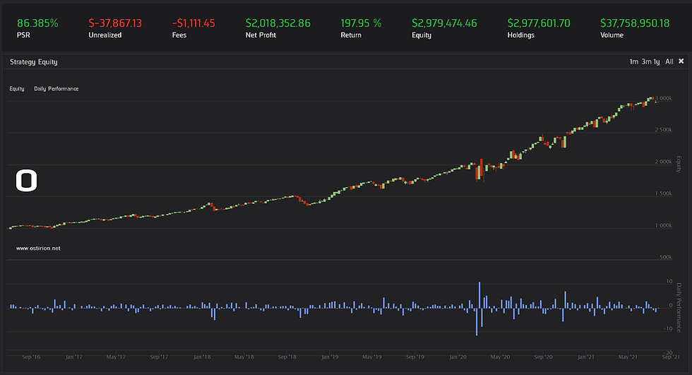
array([15, 7, 3, 18, 9, 2, 6, 17, 11, 12, 1, 19, 16, 1, 4, 14, 10, 13, 5, 8, 1, 1])Who are we to doubt the machine? Trying this random forest model we obtain the following results:

The model manages to stay at positive returns for a long time, is hit hard by some events that it can possibly not predict given the limited scope of the factors being used to predict the movements of VIX. The alpha performance indicators are good:

The alpha generates a number of directional 'hits' that is very much in line with the training results, it seems the predictive power of the fractionally differentiated SPY prices holds in time provides a small advantage over random chance.
Now the question is how do we make this slight advantage more profitable than it currently is. In the following publications we will investigate three actions to improve the trading results using this model:
Use meta-labelling to discriminate between good predictions and bad predictions even inside the "correct" predictions.
Set up prediction accuracy threshold, and trade only under those predictions that are correct, good and accurate.
Extend the model with additional factors in the same line, feeding our model with data that contains information and good statistical properties.
Remember that publications from Ostirion.net are not financial advice. Ostirion.net does not hold any positions on any of the mentioned instruments at the time of publication. If you need further information, asset management support, automated trading strategy development or tactical strategy deployment you can contact us here.

Comments