Moving Averages as Resistances and Supports

In this publication, we will walk through the implementation of the idea of using the "historically best" moving average window value as a resistance or support level for price prediction. We will reuse the model developed in our previous post and adapt it to the backtesting environment from the research environment; we will comment on what we think the critical points of the transformation are; you can always contact us or leave a comment in the post if you have some coding or LEAN-engine related question.

We are using a customized universe, altering the QC500 universe to return a variable number of symbols and be able to construct a healthily equally-weighted portfolio of large-capitalization companies that are hitting against their respective Moving Average Walls and continuing their trends. When initializing this universe baseline, we modify it so:

class CustomUniverseSelectionModel(FundamentalUniverseSelectionModel):
    def __init__(self, number, filterFineData = True, universeSettings = None, securityInitializer = None):
        '''Initializes a new default instance of the QC500UniverseSelectionModel'''super().__init__(filterFineData, universeSettings, securityInitializer)
        self.numberOfSymbolsCoarse = 1000self.numberOfSymbolsFine = number
        self.dollarVolumeBySymbol = {}
        self.lastMonth = -1

We will pass a "number" variable and expect to receive a universe with that many components at each universe selection. When these stock symbols enter the universe, they will have their "best" support/resistance moving average calculated and recorded by the adapted function we used in the research phase:

def FindBestAverage(self, history, windows):
        prices = history['close'].unstack(level=0)
        if len(prices) < 100:
            #Insufficient history length.
            return -1
        averages = prices.copy()    
        for win in windows:
            averages['MA_' + str(win)] = prices.rolling(window=win).mean()    
        averages.dropna(inplace=True)
        price_col = prices.columns[0]    
        for win in windows:
            averages['d_MA_'+str(win)] = averages[price_col] - averages['MA_' + str(win)]
            shift = averages['d_MA_'+str(win)].shift(1)
            diff = averages['d_MA_'+str(win)]
            averages['c_'+str(win)] = np.sign(shift) != np.sign(diff)     
        cross_columns = [col for col in averages.columns if 'c_' in col]    
        rates = {}    
        for column in cross_columns:
            rates[column] = averages[column].value_counts(normalize=True)[True]    
        results = {}
        for window in windows:
            results[window] = averages[[price_col, 'MA_'+str(window), 'd_MA_'+str(window),
                                        'c_'+str(window)]]    
            averages[str(window)+'_f'] = averages[price_col].shift(-window)        
            averages['ctype_'+str(window)] = averages['d_MA_'+str(window)] > 0        
            averages['FPdir_'+str(window)] = averages[str(window)+'_f'] > averages[price_col]
            averages['H_'+str(window)] = averages['ctype_'+str(window)] != averages['FPdir_'+str(window)]

            try:
                res = averages['H_'+str(window)].value_counts(normalize=True)[True]
                results[window]=res
            except:
                # There are no True values:
                results[window]=-1
          return max(results, key=results.get)   

If the history for the specific symbol is not long enough, we are going to skip that symbol; it may also be the case that there is not enough data in the series to observe resistance/support behaviors for a given moving average window, and in that case, we will return an error value of -1.

At the reception of each data update, we will check if a crossing of the price and the calculated best moving average value has happened for each of the received stock prices:

dfor s in common_list:
            if not data.get(s): continue
            s_data = self.symbol_data.get(s)
            past_status = s_data.ma_status
            current_status = data.get(s).Close > s_data.ma.Current.Value
            s_data.ma_status = data.get(s).Close > s_data.ma.Current.Value

If such a crossing has happened, we will enter the opposite position. A crossing of the moving average from below will result in a short position, a crossing from above a long position. We hypothesize that these average lines are acting as supports or resistances, and the price will rebound. Not to complicate the model too much, the duration of our prediction is symmetric to the moving average value:

period =  timedelta(days=int(s_data.best_period)) 

There is no deep rationale for this, and it may not be correct; it is just a simple assumption. We will also maintain our position until expiration; we will skip all new predictions until outstanding predictions expire. No drawdown or risk control methods are implemented; we will check how following these "most popular" moving average values, blindly, fares. The best average will be recomputed every 60 trading days period so that they are up to date and reflect the latest market action.

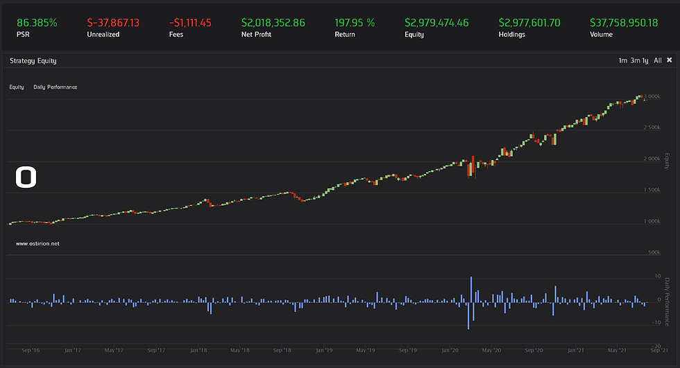
The backtest yields the following information:

Returns are not totally bad, being a stocks-only model, and even if long and short positions are allowed, the fate of the market is shared by our moving averages model. A compounding annual return of almost 11% and a Sharpe ratio of 0.85 give us some confidence in the model. It seems that for the past 5 years, there have been periods when momentum was dead, causing slight losses. When momentum is up, the model apparently picks up the correct directionality. When the market goes into crisis mode, the moving average model follows it down, many companies breach their supports and do not rebound in time.

The names that appear the most in this test are these:

Comcast, Microsoft, Visa, Amazon, and Berkshire-Hathaway generate a multitude of signals; they seem to be hitting the selected moving average lines with a high frequency. These signals have this appearance at the middle of the test:

A mix of long and short positions, with various moving average values as both signal and duration. The long and short positions are not controlled whatsoever, nor is the minimum quantity of signals to be generated. The model can generate some risky individual trades that we are not looking at and could be controlled. There seems to be some pattern to these moving averages as resistances and supports, the directionality of the price movement is captured slightly above 55%, and most of the misses come from the beginning of 2020 and the COVID19 crisis, which destroyed momentum, among other things:

The model does not perform horribly; it is very wild and seems to pick up simple momentum quite well. It surely requires more work in terms of risk balancing and absurd positioning prevention. In future posts, we will try to add some control and balance; a handy beta finding function is added in the research file of the attached backtest example; we will use it:

Information in ostirion.net does not constitute financial advice; we do not hold positions in any of the companies or assets that we mention in our posts at the time of posting. If you require quantitative model development, deployment, verification, or validation, do not hesitate and contact us. We will also be glad to help you with your machine learning or artificial intelligence challenges when applied to asset management, trading, or risk evaluations.